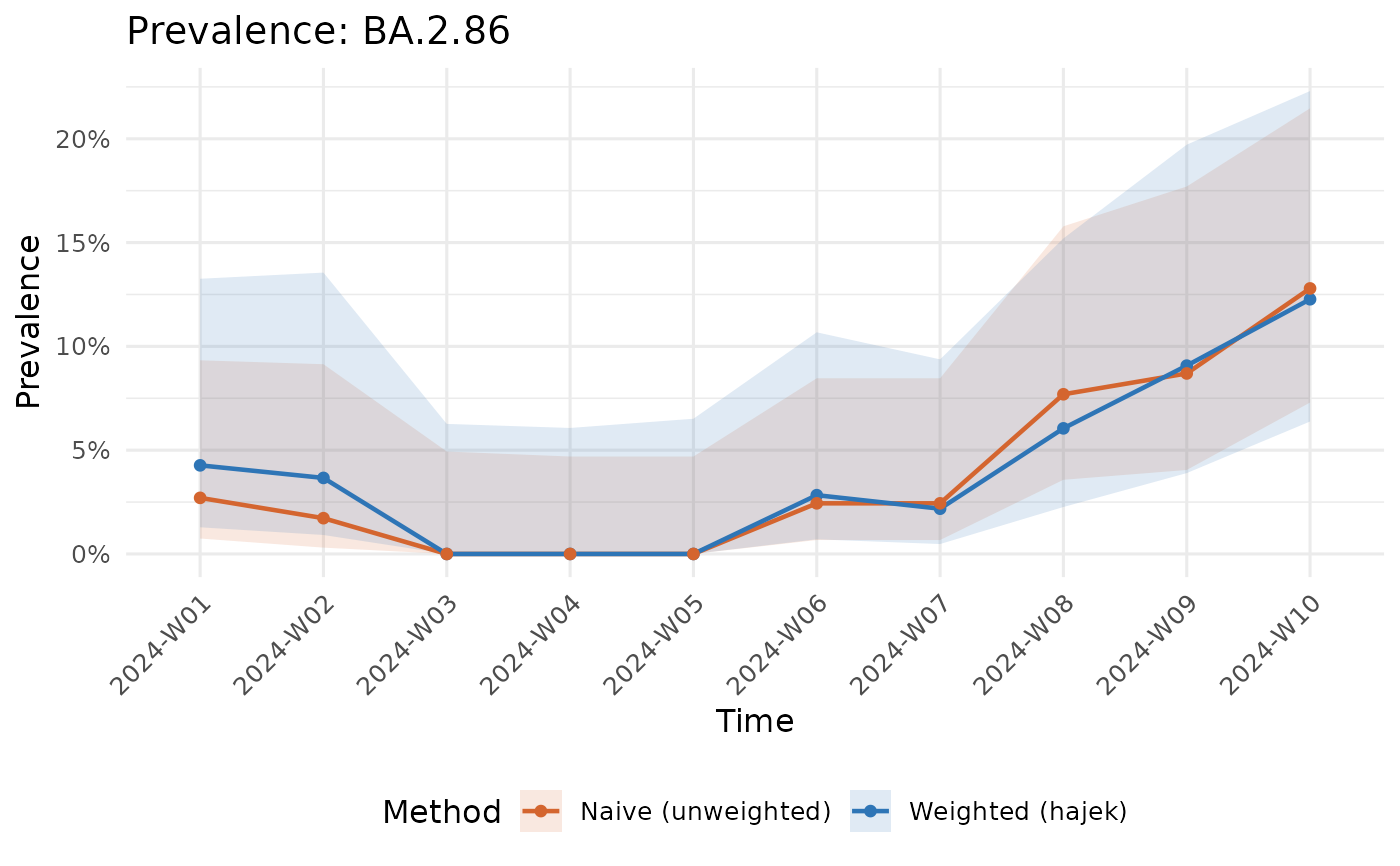
Compare weighted vs naive prevalence estimates — surv_compare_estimates • survinger

Side-by-side plot showing the impact of design correction.

Usage

surv_compare_estimates(weighted, naive, title = NULL)

Arguments

weighted: A surv_prevalence object (design-weighted).
naive: A surv_prevalence object (unweighted).
title: Character or NULL. Plot title.

Value

A ggplot2 object.

Examples

sim <- surv_simulate(n_regions = 3, n_weeks = 10, seed = 1)
d <- surv_design(sim$sequences, ~ region,
                 sim$population[c("region", "seq_rate")], sim$population)
w <- surv_lineage_prevalence(d, "BA.2.86")
n <- surv_naive_prevalence(d, "BA.2.86")
surv_compare_estimates(w, n)