Overview
lineagefreq provides multiple modeling engines through the unified
fit_model() interface. This vignette shows how to compare
them using the built-in backtesting framework.
Three engines are available in v0.1.0:
- mlr: Multinomial logistic regression (frequentist, fast).
- piantham: Converts MLR growth rates to relative reproduction numbers using a generation-time approximation.
- hier_mlr: Hierarchical MLR with partial pooling across locations via empirical Bayes shrinkage.
Engine 1: MLR
The default engine fits a multinomial logistic regression with one growth rate parameter per non-reference lineage.
data(sarscov2_us_2022)
x <- lfq_data(sarscov2_us_2022,
              lineage = variant, date = date,
              count = count, total = total)

fit_mlr <- fit_model(x, engine = "mlr")
growth_advantage(fit_mlr, type = "growth_rate")
#> # A tibble: 5 × 6
#>   lineage estimate lower upper type        pivot
#>   <chr>      <dbl> <dbl> <dbl> <chr>       <chr>
#> 1 BA.1       0     0     0     growth_rate BA.1
#> 2 BA.2       0.231 0.229 0.232 growth_rate BA.1
#> 3 BA.4/5     0.400 0.398 0.402 growth_rate BA.1
#> 4 BQ.1       0.352 0.346 0.357 growth_rate BA.1
#> 5 Other      0.151 0.149 0.152 growth_rate BA.1
Engine 2: Piantham
The Piantham engine wraps MLR and translates growth rates to relative effective reproduction numbers using a specified mean generation time.
fit_pian <- fit_model(x, engine = "piantham",
                      generation_time = 5)
growth_advantage(fit_pian, type = "relative_Rt",
                 generation_time = 5)
#> # A tibble: 5 × 6
#>   lineage estimate lower upper type        pivot
#>   <chr>      <dbl> <dbl> <dbl> <chr>       <chr>
#> 1 BA.1        1     1     1    relative_Rt BA.1
#> 2 BA.2        1.18  1.18  1.18 relative_Rt BA.1
#> 3 BA.4/5      1.33  1.33  1.33 relative_Rt BA.1
#> 4 BQ.1        1.29  1.28  1.29 relative_Rt BA.1
#> 5 Other       1.11  1.11  1.11 relative_Rt BA.1
Comparing fit statistics
glance() returns a one-row summary for each model. Since
Piantham is a wrapper around MLR, the log-likelihood and AIC are
identical.
dplyr::bind_rows(
  glance.lfq_fit(fit_mlr),
  glance.lfq_fit(fit_pian)
)
#> # A tibble: 2 × 10
#>   engine   n_lineages n_timepoints   nobs    df   logLik     AIC     BIC pivot
#>   <chr>         <int>        <int>  <int> <int>    <dbl>   <dbl>   <dbl> <chr>
#> 1 mlr               5           40 461424     8 -465911. 931838. 931852. BA.1
#> 2 piantham          5           40 461424     8 -465911. 931838. 931852. BA.1
#> # ℹ 1 more variable: convergence <int>
Backtesting
The backtest() function implements rolling-origin
evaluation. At each origin date, the model is fit on past data and
forecasts are compared to held-out future observations.
bt <- backtest(x,
  engines = c("mlr", "piantham"),
  horizons = c(7, 14, 21),
  min_train = 56,
  generation_time = 5
)
#> Backtesting ■■■                                7% | ETA: 14s
#> Backtesting ■■■■■■■■■                         26% | ETA: 11s
#> Backtesting ■■■■■■■■■■■■■■                    42% | ETA: 10s
#> Backtesting ■■■■■■■■■■■■■■■■■■                55% | ETA:  8s
#> Backtesting ■■■■■■■■■■■■■■■■■■■■■■            70% | ETA:  6s
#> Backtesting ■■■■■■■■■■■■■■■■■■■■■■■■■         81% | ETA:  4s
#> Backtesting ■■■■■■■■■■■■■■■■■■■■■■■■■■■■■     92% | ETA:  2s
#> Backtesting ■■■■■■■■■■■■■■■■■■■■■■■■■■■■■■■  100% | ETA:  0s
bt
#>
#> ── Backtest results
#> 900 predictions across 31 origins
#> Engines: "mlr, piantham"
#> Horizons: 7, 14, 21 days
#>
#> # A tibble: 900 × 9
#>    origin_date target_date horizon engine lineage predicted lower  upper
#>  * <date>      <date>        <int> <chr>  <chr>       <dbl> <dbl>  <dbl>
#>  1 2022-03-05  2022-03-12        7 mlr    BA.1         0.44  0.34 0.53
#>  2 2022-03-05  2022-03-12        7 mlr    BA.2         0.18  0.11 0.26
#>  3 2022-03-05  2022-03-12        7 mlr    BA.4/5       0     0    0.02
#>  4 2022-03-05  2022-03-12        7 mlr    BQ.1         0     0    0.01
#>  5 2022-03-05  2022-03-12        7 mlr    Other        0.37  0.28 0.47
#>  6 2022-03-05  2022-03-19       14 mlr    BA.1         0.4   0.31 0.5
#>  7 2022-03-05  2022-03-19       14 mlr    BA.2         0.21  0.13 0.29
#>  8 2022-03-05  2022-03-19       14 mlr    BA.4/5       0     0    0.0252
#>  9 2022-03-05  2022-03-19       14 mlr    BQ.1         0     0    0.01
#> 10 2022-03-05  2022-03-19       14 mlr    Other        0.39  0.29 0.49
#> # ℹ 890 more rows
#> # ℹ 1 more variable: observed <dbl>
Scoring
score_forecasts() computes standardized accuracy
metrics.
sc <- score_forecasts(bt,
  metrics = c("mae", "coverage"))
sc
#> # A tibble: 12 × 4
#>    engine   horizon metric     value
#>    <chr>      <int> <chr>      <dbl>
#>  1 mlr            7 mae      0.00399
#>  2 mlr            7 coverage 1
#>  3 mlr           14 mae      0.00436
#>  4 mlr           14 coverage 1
#>  5 mlr           21 mae      0.00447
#>  6 mlr           21 coverage 1
#>  7 piantham       7 mae      0.00441
#>  8 piantham       7 coverage 0.994
#>  9 piantham      14 mae      0.00448
#> 10 piantham      14 coverage 1
#> 11 piantham      21 mae      0.00447
#> 12 piantham      21 coverage 0.993
Model ranking
compare_models() summarizes scores per engine, sorted by
MAE.
compare_models(sc, by = c("engine", "horizon"))
#> # A tibble: 6 × 4
#>   engine   horizon     mae coverage
#>   <chr>      <int>   <dbl>    <dbl>
#> 1 mlr            7 0.00399    1
#> 2 mlr           14 0.00436    1
#> 3 piantham       7 0.00441    0.994
#> 4 mlr           21 0.00447    1
#> 5 piantham      21 0.00447    0.993
#> 6 piantham      14 0.00448    1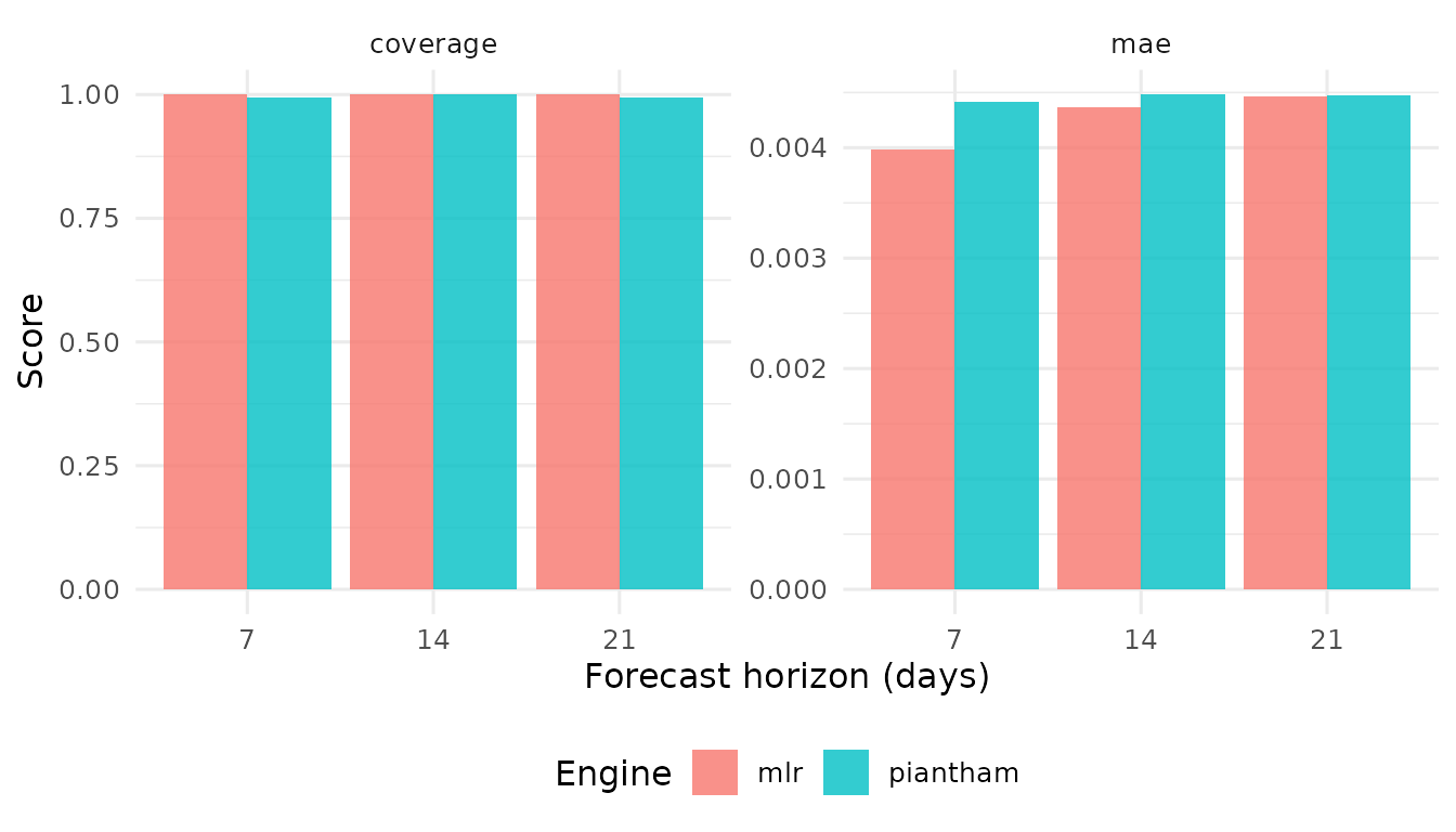
When to use which engine
| Scenario | Recommended engine |
|---|---|
| Single location, quick estimate | mlr |
| Need relative Rt interpretation | piantham |
| Multiple locations, sparse data | hier_mlr |
| Time-varying fitness (v0.2) | garw |
Hierarchical MLR
When data spans multiple locations with unequal sequencing depth,
hier_mlr shrinks location-specific estimates toward the
global mean. This stabilizes estimates for low-data locations.
A demonstration requires multi-location data, which the built-in
single-location dataset does not provide. See ?fit_model
for an example with simulated multi-location data.