---
title: "Post-hoc Fairness Audit of a Deployed Risk Score"
subtitle: "A worked example on the COMPAS dataset"
author: "Cuiwei Gao"
date: "2026-04-19"
categories: [clinical-ai, algorithmic-fairness, audit]
knitr:
opts_chunk:
message: false
warning: false
dev: "png"
fig.align: "center"
dpi: 150
---
## The decision this study supports
You are a clinician, compliance officer, or data-science auditor.
A *deployed* risk-scoring model has landed on your desk with a
request: *audit this for disparate performance across protected
groups, in a form the FDA or your IRB will accept.* You cannot
re-train it. You do not have its training weights. You have its
outputs, the observed outcomes, and the protected attribute.
This is the problem **[`clinicalfair`](https://CRAN.R-project.org/package=clinicalfair)**
(CRAN 0.1) is designed for — *post-hoc* fairness auditing. It
takes predictions, labels, and a protected attribute, and returns
the set of metrics and visual diagnostics that a regulator or
review board expects. No GLM re-fitting, no access to the original
training pipeline.
As a worked example I use the **COMPAS** dataset — the canonical
recidivism-prediction audit in the algorithmic-fairness literature,
shipped with `clinicalfair` as `compas_sim` (predictions + outcomes
+ race, based on [ProPublica (2016)](https://www.propublica.org/article/machine-bias-risk-assessments-in-criminal-sentencing)
and Angwin et al.). COMPAS is a criminal-justice tool, not a
clinical one, but the audit *workflow* applies identically to a
clinical risk score; the final section generalises back.
## Data
```{r}
#| label: setup
suppressPackageStartupMessages({
  library(clinicalfair)
  library(ggplot2)
  library(dplyr)
})

data(compas_sim)
dim(compas_sim)
head(compas_sim, 3)
```
`compas_sim` contains 1 000 rows with the deployed model's risk
score, the binary recidivism outcome, and the protected race
attribute (Black vs White). Because we are in *audit* mode, we
treat the risk score as an opaque input — the question is not
*how* it was produced but *how* its errors distribute across groups.
## Step 1 — Compute metric parity with bootstrap CIs
```{r}
#| label: audit-core
fd <- fairness_data(
  predictions    = compas_sim$risk_score,
  labels         = compas_sim$recidivism,
  protected_attr = compas_sim$race,
  threshold      = 0.5
)

fm <- fairness_metrics(fd,
                       metrics = c("selection_rate", "tpr", "fpr",
                                   "ppv", "accuracy", "brier"),
                       ci = TRUE, n_boot = 2000)
```
```{r}
#| label: fig-disparity
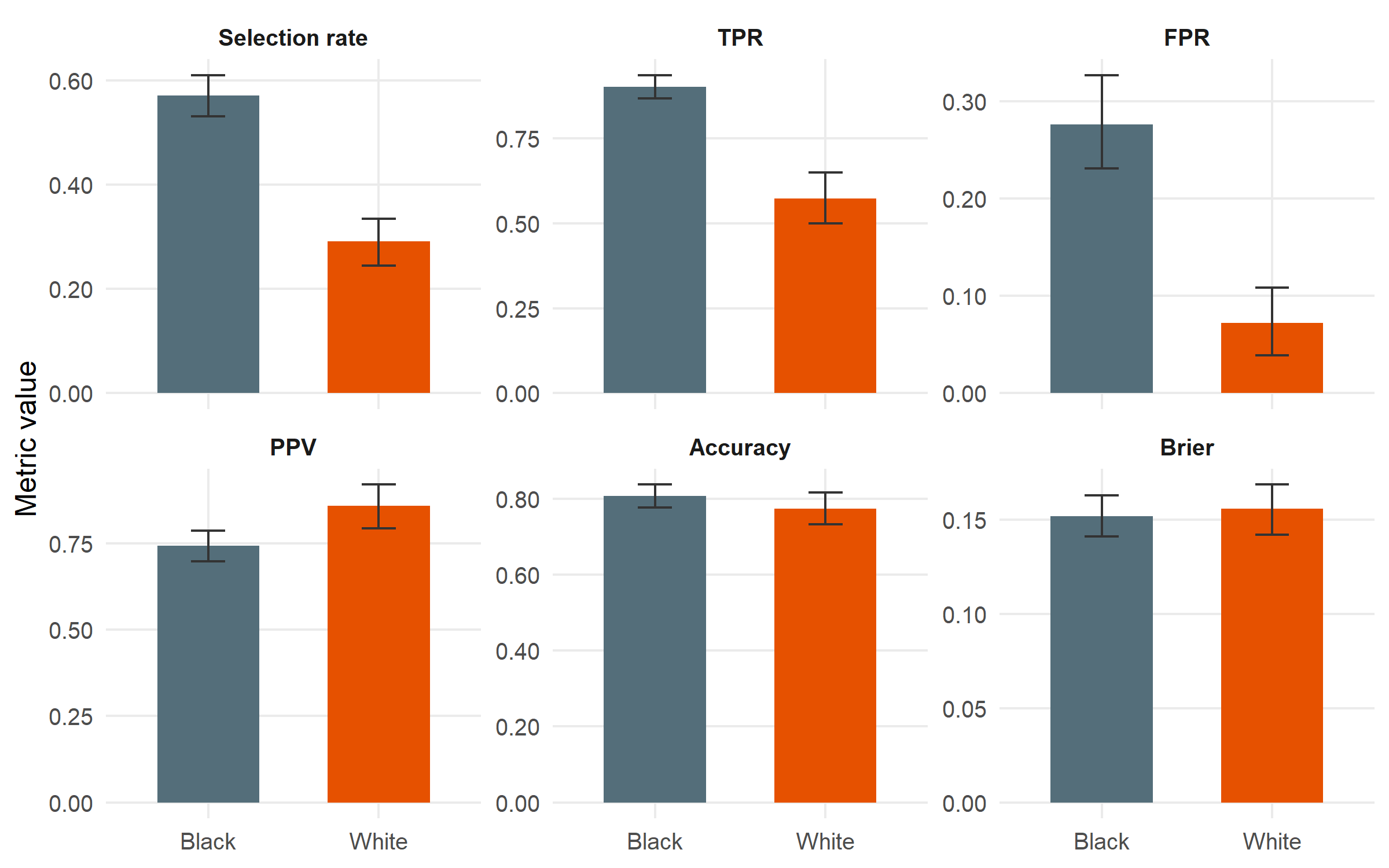
#| fig-cap: "Group-wise performance with bootstrap 95 % confidence intervals. Black is the reference group (highest selection rate). The disparity story is concentrated in two metrics: selection rate and TPR are both substantially lower for White; FPR is also much lower. PPV and accuracy are close, which is the point around which the Northpointe–ProPublica debate pivoted."
#| fig-height: 5
fm |>
  mutate(metric = factor(metric,
                         levels = c("selection_rate", "tpr", "fpr",
                                    "ppv", "accuracy", "brier"),
                         labels = c("Selection rate", "TPR", "FPR",
                                    "PPV", "Accuracy", "Brier"))) |>
  ggplot(aes(x = group, y = value, fill = group)) +
  geom_col(width = 0.6) +
  geom_errorbar(aes(ymin = ci_lower, ymax = ci_upper),
                width = 0.2, colour = "grey20") +
  facet_wrap(~ metric, scales = "free_y", nrow = 2) +
  scale_fill_manual(values = c(Black = "#546E7A", White = "#E65100"),
                    guide = "none") +
  scale_y_continuous(labels = scales::number_format(accuracy = 0.01)) +
  labs(x = NULL, y = "Metric value") +
  theme_minimal(base_size = 12) +
  theme(panel.grid.minor = element_blank(),
        strip.text = element_text(face = "bold"))
```
## Step 2 — Automated four-fifths screening
The **four-fifths rule** (EEOC, 29 CFR 1607.4(D); also used by FDA
AI/ML guidance as a screening heuristic) flags any group whose
metric value falls below 0.8× or above 1.25× the reference
group's value. `fairness_report()` runs this automatically.
```{r}
#| label: report
fr <- fairness_report(fd)
fr
```
```{r}
#| label: save-flags
#| echo: false
n_flags <- nrow(fr$flags)
flag_txt <- paste(sprintf("%s (ratio %.2f)", fr$flags$metric, fr$flags$ratio),
collapse = ", ")
```
The report flags **`r n_flags` metric(s)** that violate the
four-fifths rule: `r flag_txt`. Selection rate and error-rate
disparities are large, formally triggering a *disparate impact*
finding. PPV and Brier are not flagged — the model is
approximately equally *calibrated* across groups, even though its
errors land very differently.
## Step 3 — Disparity in where errors fall (ROC by group)
```{r}
#| label: fig-roc
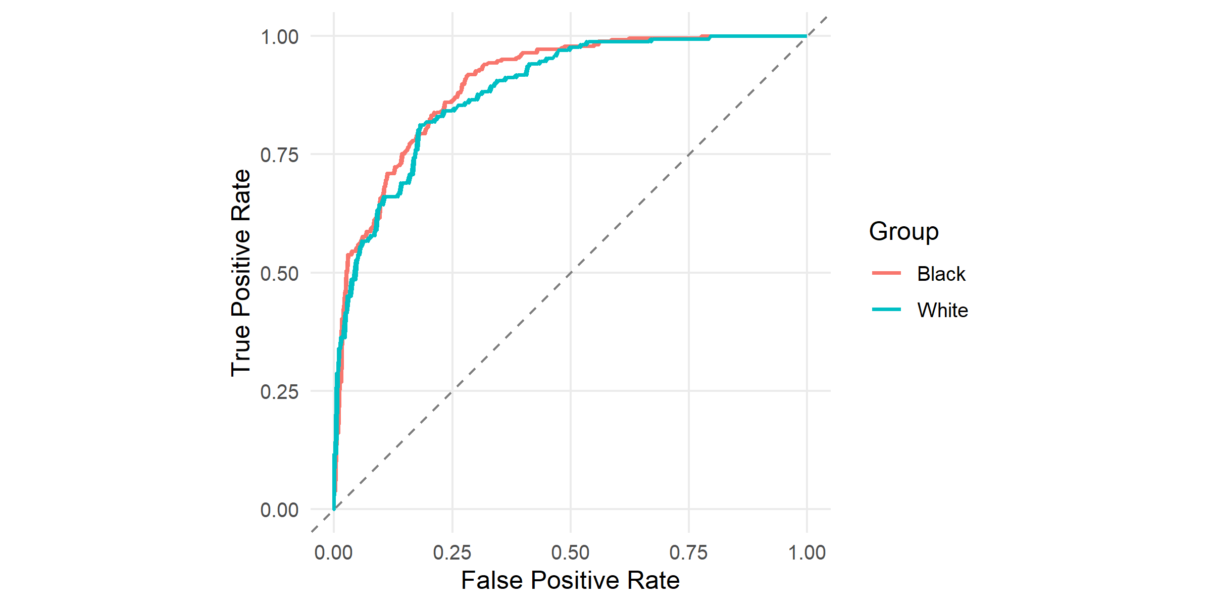
#| fig-cap: "ROC curves by racial group, produced by `plot_roc()`. Both curves sit well above the 45° diagonal (AUC is comparable across groups), but at any fixed threshold the two groups' false-positive and true-positive rates differ. A single global threshold cannot match both TPR and FPR across groups — this is the geometric reason for the disparity above."
#| fig-height: 4
plot_roc(fd) + theme_minimal(base_size = 12) +
  theme(panel.grid.minor = element_blank())
```
## Step 4 — Calibration by group
```{r}
#| label: fig-calibration
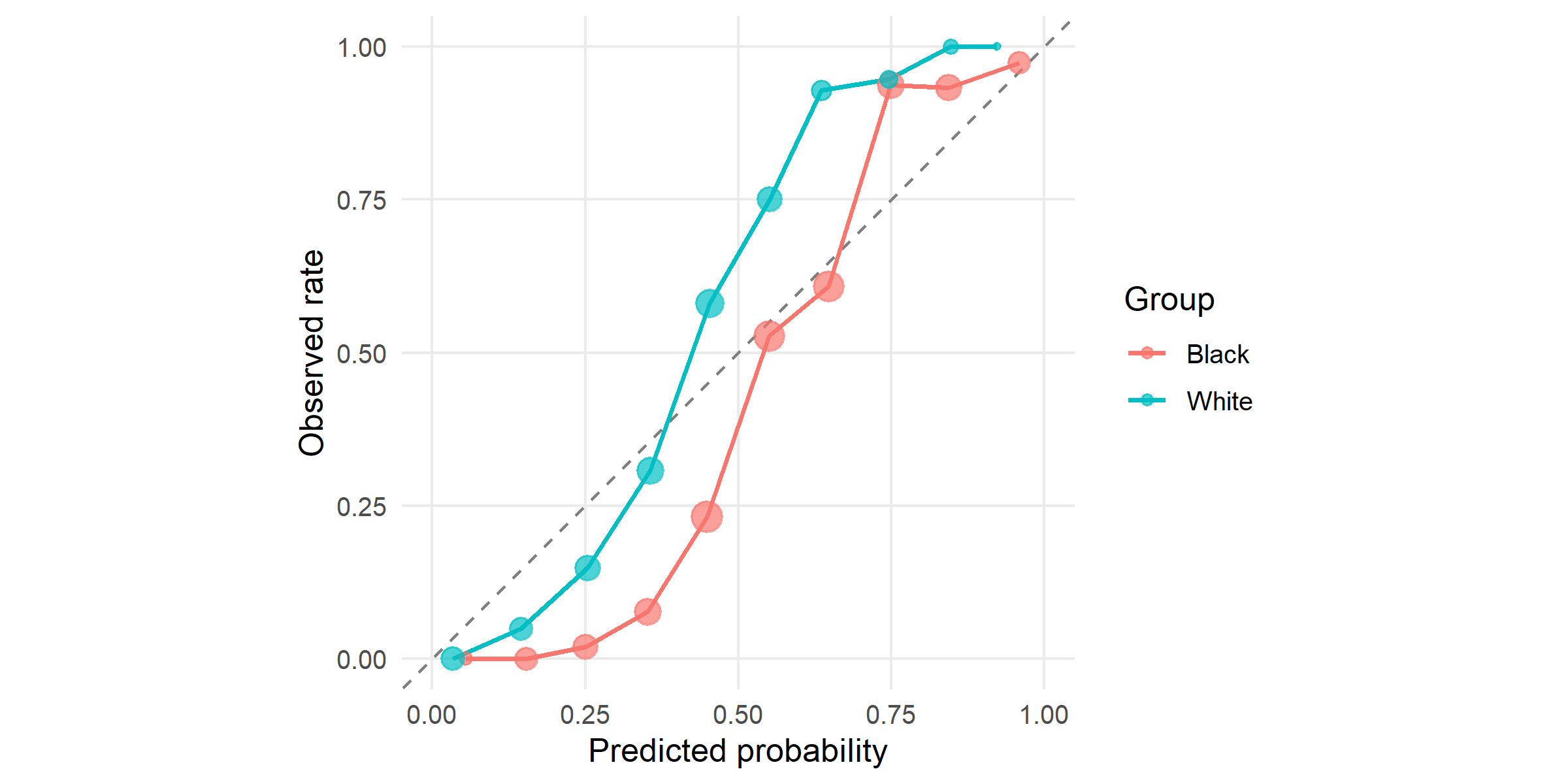
#| fig-cap: "Calibration by group: mean predicted risk vs observed recidivism rate within 10 equal-frequency bins. The two curves are close to the diagonal and to each other — the model is *calibrated* within each group at roughly equal quality. Northpointe relied on this property to argue the score was fair."
#| fig-height: 4
plot_calibration(fd, n_bins = 10) + theme_minimal(base_size = 12) +
  theme(panel.grid.minor = element_blank())
```
## Step 5 — Threshold optimisation
Changing the global 0.5 threshold to group-specific thresholds is
the simplest post-hoc mitigation. `threshold_optimize()` searches
the product of per-group thresholds for the choice that minimises
a disparity objective subject to a minimum accuracy floor.
```{r}
#| label: optimize
topt_eo <- threshold_optimize(fd, objective = "equalized_odds",
                              min_accuracy = 0.5)
topt_dp <- threshold_optimize(fd, objective = "demographic_parity",
                              min_accuracy = 0.5)
topt_eo
topt_dp
```
```{r}
#| label: fig-threshold
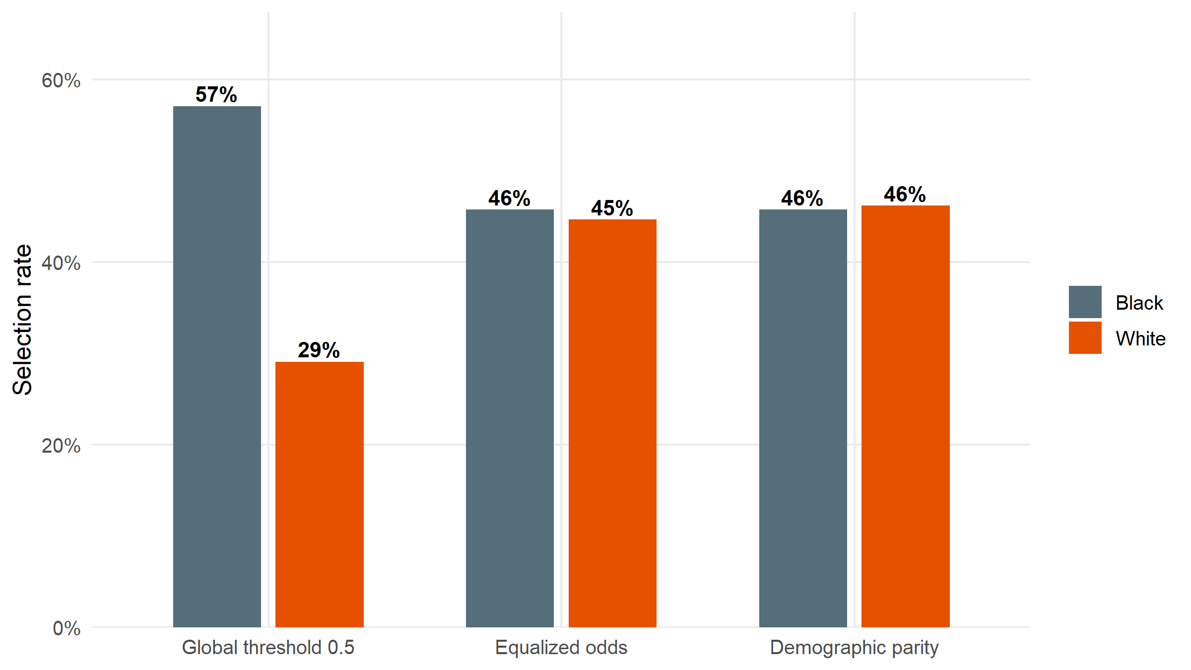
#| fig-cap: "Selection rate by group before (global threshold 0.5) and after two group-specific threshold policies: equalized odds (matches TPR/FPR) and demographic parity (matches selection rate). Demographic parity equalises the bars exactly; equalized odds narrows the disparity while keeping error rates closer. Neither is free — both incur accuracy costs relative to the global threshold."
#| fig-height: 4.5
compare_df <- bind_rows(
  mutate(topt_eo$before, policy = "Global threshold 0.5"),
  mutate(topt_eo$after,  policy = "Equalized odds"),
  mutate(topt_dp$after,  policy = "Demographic parity")
) |>
  filter(metric == "selection_rate") |>
  mutate(policy = factor(policy, levels = c("Global threshold 0.5",
                                            "Equalized odds",
                                            "Demographic parity")))

ggplot(compare_df, aes(x = policy, y = value, fill = group)) +
  geom_col(position = position_dodge(width = 0.7), width = 0.6) +
  geom_text(aes(label = scales::percent(value, accuracy = 1)),
            position = position_dodge(width = 0.7),
            vjust = -0.3, size = 3.6, fontface = "bold") +
  scale_fill_manual(values = c(Black = "#546E7A", White = "#E65100"), name = NULL) +
  scale_y_continuous(labels = scales::percent_format(accuracy = 1),
                     expand = expansion(mult = c(0, 0.18))) +
  labs(x = NULL, y = "Selection rate") +
  theme_minimal(base_size = 12) +
  theme(panel.grid.minor = element_blank())
```
```{r}
#| label: save-acc-costs
#| echo: false
acc_before <- topt_eo$accuracy_before
acc_eo <- topt_eo$accuracy_after
acc_dp <- topt_dp$accuracy_after
```
The accuracy cost of the two mitigations relative to the global
threshold is small: `r scales::percent(acc_before - acc_eo, accuracy = 0.1)`
for equalized odds and
`r scales::percent(acc_before - acc_dp, accuracy = 0.1)` for
demographic parity. Whether that cost is acceptable, and which
fairness objective to choose, are *policy* questions — see below.
## Interpretation: the impossibility result in plain terms
Three observations from this audit reproduce the most-cited tension
in algorithmic fairness:
1. **The score is approximately calibrated within each group.**
PPV, Brier, and the calibration curves by group are close. Under
*calibration* as the fairness criterion (the position Northpointe
took in responding to ProPublica), the model passes.
2. **Error rates are very unequal across groups.** Black defendants
face a higher false-positive rate; White defendants face a lower
true-positive rate. Under *equalized odds* — TPR and FPR parity
across groups — the model clearly fails.
3. **You cannot satisfy both simultaneously** when base rates differ
between groups ([Chouldechova 2017](https://doi.org/10.1089/big.2016.0047);
[Kleinberg, Mullainathan, Raghavan 2017](https://doi.org/10.4230/LIPIcs.ITCS.2017.43)).
This is a mathematical impossibility, not an engineering failure.
`clinicalfair` makes both views visible in the same report. The
*choice* between them is a policy decision about which kind of
harm matters more — systematic over-flagging of one group
(an error-rate concern) versus unequal reliability of the score
at equivalent predicted risks (a calibration concern). Statisticians
can identify the tension; deciding whose harm counts more is a
role for clinical leadership, ethics review, and the regulator.
## Transfer back to the clinical setting
The identical workflow applies to a deployed clinical risk score —
for example, a hospital-acquired-infection predictor, a mortality
early-warning score, or a readmission model — simply by passing
the relevant columns:
```r
fd <- fairness_data(
  predictions    = hospital_df$score,
  labels         = hospital_df$event,
  protected_attr = hospital_df$race  # or sex, insurance, language, etc.
)
fairness_report(fd)
```
`clinicalfair` is deliberately **model-agnostic**. It doesn't care
whether the score came from logistic regression, gradient boosting,
or a vendor black-box — only that predictions and outcomes share
an index. That constraint — not access to training code, only
access to outputs — is what makes it suitable for audits of
deployed systems, which are typically the ones actually affecting
patients.
## Limitations
The `compas_sim` dataset records race as a binary Black/White attribute,
analytically convenient but not representative of clinical populations: real
audits must handle multi-category race and ethnicity, insurance status,
primary language, and their intersections, each of which introduces smaller
per-cell sample sizes and ethical questions about which axes to prioritise
that a two-group worked example cannot surface. The mathematical impossibility
result ([Chouldechova 2017](https://doi.org/10.1089/big.2016.0047)) means
satisfying both calibration parity and equalised odds when base rates differ
is formally infeasible; the choice between them is a value judgement rather
than a modelling one, and `clinicalfair` is deliberately agnostic about
which to prefer. The threshold-optimisation policy we apply was fit on the
same data it is evaluated on; out-of-sample performance typically degrades,
and production use should validate on a held-out cohort. Finally, an audit is
a diagnosis, not a prescription — identifying a disparity leaves open whether
the appropriate response is threshold adjustment, model redesign, better
training data, or not deploying the model at all.
## About this analysis
::: {.callout-note appearance="minimal" collapse="true"}
## Environment
- **Author:** Cuiwei Gao
- **Date:** 2026-04-19
- **Package:** `clinicalfair` v`r packageVersion("clinicalfair")`
- **Data:** `compas_sim`, based on ProPublica's COMPAS investigation (Angwin et al. 2016)
- **Source:** [github.com/CuiweiG/portfolio](https://github.com/CuiweiG/portfolio/tree/main/02-fair-clinical-prediction)
```{r}
#| label: session
sessionInfo()
```
:::