---
title: "Releasing Synthetic Clinical Data"
subtitle: "A privacy-utility analysis across three synthesis methods"
author: "Cuiwei Gao"
date: "2026-04-19"
categories: [clinical-data, synthetic-data, privacy, data-sharing]
knitr:
opts_chunk:
message: false
warning: false
dev: "png"
fig.align: "center"
dpi: 150
---
## Motivation
A research consortium wants to release a patient cohort to external
collaborators. HIPAA and equivalent non-US frameworks block direct
release. The consortium considers a **synthetic** surrogate — a
dataset with the statistical texture of the original but no
one-to-one mapping to any real patient. Three questions determine
whether this is a safe release:
1. **Does the synthetic data still carry the real-data signal?**
Means, variances, and (crucially) correlations must be
preserved or downstream analyses will reach different conclusions.
2. **Is it safe?** Can an adversary link a synthetic record back to
a specific patient? How close are synthetic records to real ones?
3. **Which synthesis method is right for this use case?**
This case study applies **[`syntheticdata`](https://CRAN.R-project.org/package=syntheticdata)**
(CRAN 0.1) to a simulated clinical cohort — comparing Gaussian
copula, bootstrap-with-noise, and Laplace-noise synthesis against a
shared utility-and-privacy scorecard, and then mapping the three
methods onto a privacy-utility Pareto frontier.
## Data
Because the point of this study *is* data release, the "real" cohort
here is itself simulated — a 500-patient clinical-like dataset
whose distributions and correlations match the kind of cohort a
cardiology trial might collect (age, SBP, BMI, glucose, LDL, and a
30-day readmission outcome). Everything downstream treats it as the
real data.
```{r}
#| label: setup
suppressPackageStartupMessages({
  library(syntheticdata)
  library(ggplot2)
  library(dplyr)
  library(tidyr)
})

set.seed(42)
n <- 500
real <- data.frame(
  age     = pmax(35, pmin(90,  rnorm(n, 65,  10))),
  sbp     = pmax(85, pmin(200, rnorm(n, 132, 18))),
  bmi     = pmax(17, pmin(45,  rnorm(n, 28,   5))),
  glucose = pmax(65, pmin(280, rnorm(n, 98,  22))),
  ldl     = pmax(40, pmin(220, rnorm(n, 115, 28)))
)
# A correlated binary outcome (higher risk with higher SBP and glucose)
lp <- scale(real$sbp)[, 1] * 0.6 + scale(real$glucose)[, 1] * 0.4 - 2
real$readmit_30d <- rbinom(n, 1, plogis(lp))

glimpse(real)
```
```{r}
#| label: real-summary
#| echo: false
real |>
summarise(across(c(age, sbp, bmi, glucose, ldl),
list(mean = \(x) round(mean(x), 1),
sd = \(x) round(sd(x), 1)),
.names = "{.col}__{.fn}")) |>
pivot_longer(everything(),
names_to = c("variable", ".value"),
names_sep = "__")
```
## Step 1 — Generate synthetic data with three methods
```{r}
#| label: synthesize
syn_para <- synthesize(real, method = "parametric", seed = 42)
syn_boot <- synthesize(real, method = "bootstrap",  seed = 42)
syn_nois <- synthesize(real, method = "noise",      seed = 42)
```
Three distinct strategies:
- `parametric` fits a Gaussian copula to the continuous variables
and a multinomial model to categoricals, preserving marginal
distributions and pairwise dependence.
- `bootstrap` resamples rows with replacement, optionally adding
small noise — preserves joint distribution exactly but exposes
record-level similarity to the real data.
- `noise` adds Laplace noise calibrated to each variable's scale
(a differential-privacy-inspired mechanism).
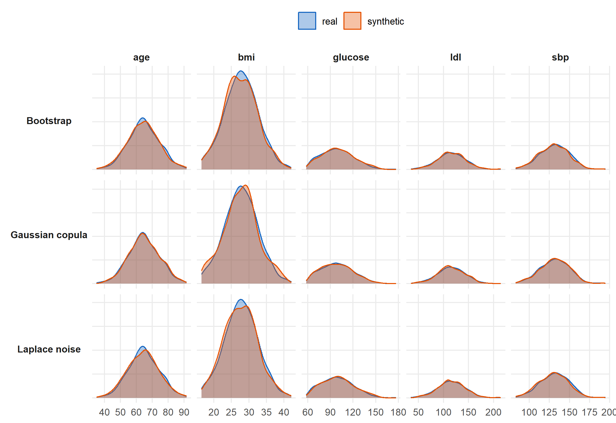
## Step 2 — Marginal fidelity
```{r}
#| label: fig-distributions
#| fig-cap: "Real vs synthetic marginal distributions across all five continuous variables, for each of the three methods. Solid = real, outlined = synthetic. The Gaussian copula tracks each marginal tightly; bootstrap preserves shape (by construction); Laplace noise inflates tails."
#| fig-height: 5.5
combine_syn <- function(real, syn, method_label) {
  bind_rows(
    mutate(real, source = "real"),
    mutate(syn$synthetic, source = "synthetic")
  ) |>
    select(age, sbp, bmi, glucose, ldl, source) |>
    pivot_longer(-source, names_to = "variable", values_to = "value") |>
    mutate(method = method_label)
}

all_df <- bind_rows(
  combine_syn(real, syn_para, "Gaussian copula"),
  combine_syn(real, syn_boot, "Bootstrap"),
  combine_syn(real, syn_nois, "Laplace noise")
)

ggplot(all_df, aes(x = value, fill = source, colour = source)) +
  geom_density(alpha = 0.35, linewidth = 0.5) +
  facet_grid(method ~ variable, scales = "free", switch = "y") +
  scale_fill_manual(values = c(real = "#1565C0", synthetic = "#E65100"),
                    name = NULL) +
  scale_colour_manual(values = c(real = "#1565C0", synthetic = "#E65100"),
                      name = NULL) +
  labs(x = NULL, y = NULL) +
  theme_minimal(base_size = 11) +
  theme(panel.grid.minor = element_blank(),
        strip.text.y.left = element_text(angle = 0, face = "bold"),
        strip.text.x = element_text(face = "bold"),
        axis.text.y = element_blank(),
        legend.position = "top")
```
## Step 3 — Multi-metric scorecard
`compare_methods()` runs all three synthesis methods against the
same real data and computes a unified validation tibble: KS fidelity,
correlation preservation, discriminative AUC (a classifier trained
to tell real from synthetic — ideally ≈ 0.5), and nearest-neighbor
distance ratio (> 1 means synthetic records are not closer to real
records than real records are to each other).
```{r}
#| label: compare
cmp <- compare_methods(real, seed = 42)
```
```{r}
#| label: tbl-compare
#| echo: false
cmp |>
mutate(value = round(value, 3)) |>
pivot_wider(id_cols = method, names_from = metric, values_from = value) |>
arrange(method) |>
knitr::kable(caption = "Unified utility + privacy scorecard from `compare_methods()`.")
```
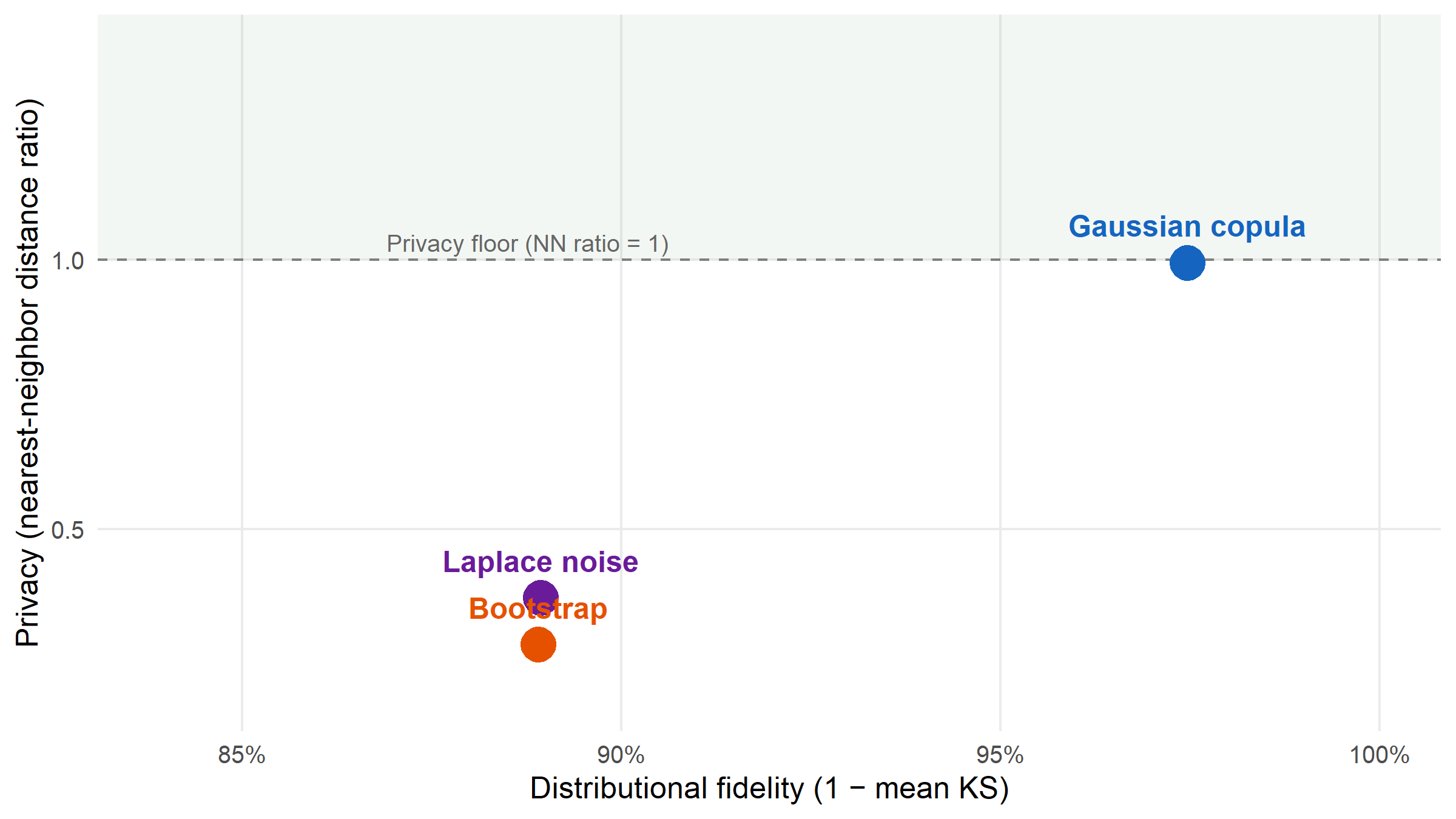
## Step 4 — Privacy-utility Pareto plot
```{r}
#| label: fig-pareto
#| fig-cap: "Each synthesis method as a point on a privacy–utility plane. X axis: distributional fidelity (1 − mean KS; higher = better utility). Y axis: nearest-neighbor distance ratio (higher = safer). The dashed line at 1 is the privacy floor: synthetic records start to look closer to real records than real-to-real when below it. The Gaussian copula sits highest in privacy with negligible utility penalty relative to bootstrap; Laplace noise and bootstrap crowd into the low-privacy region."
#| fig-height: 4.5
ks_df <- cmp |> filter(metric == "ks_statistic_mean") |>
  transmute(method, fidelity = 1 - value)
nn_df <- cmp |> filter(metric == "nn_distance_ratio") |>
  transmute(method, privacy = value)
auc_df <- cmp |> filter(metric == "discriminative_auc") |>
  transmute(method, disc_auc = value)
corr_df <- cmp |> filter(metric == "correlation_diff") |>
  transmute(method, corr_diff = value)
plot_df <- ks_df |>
  left_join(nn_df,   by = "method") |>
  left_join(auc_df,  by = "method") |>
  left_join(corr_df, by = "method") |>
  mutate(label = recode(method,
                        parametric = "Gaussian copula",
                        bootstrap  = "Bootstrap",
                        noise      = "Laplace noise"))

ggplot(plot_df, aes(x = fidelity, y = privacy, colour = method)) +
  annotate("rect", xmin = -Inf, xmax = Inf, ymin = 1, ymax = Inf,
           fill = "#2E7D32", alpha = 0.06) +
  geom_hline(yintercept = 1, linetype = "dashed", colour = "grey50") +
  geom_point(size = 6) +
  geom_text(aes(label = label), vjust = -1.2, fontface = "bold",
            size = 4.1, show.legend = FALSE) +
  annotate("text",
           x = min(plot_df$fidelity) - 0.02, y = 1,
           label = "Privacy floor (NN ratio = 1)",
           hjust = 0, vjust = -0.5, size = 3.3, colour = "grey40") +
  scale_colour_manual(values = c(parametric = "#1565C0",
                                 bootstrap  = "#E65100",
                                 noise      = "#6A1B9A"),
                      guide = "none") +
  scale_x_continuous(labels = scales::percent_format(accuracy = 1),
                     limits = c(min(plot_df$fidelity) - 0.05, 1)) +
  scale_y_continuous(limits = c(min(plot_df$privacy, na.rm = TRUE) - 0.1,
                                max(plot_df$privacy, na.rm = TRUE) + 0.4)) +
  labs(x = "Distributional fidelity (1 − mean KS)",
       y = "Privacy (nearest-neighbor distance ratio)") +
  theme_minimal(base_size = 12) +
  theme(panel.grid.minor = element_blank())
```
## Step 5 — Does the synthetic data preserve predictive signal?
A privacy-preserving synthetic dataset is useless if downstream
modelling on it gives different answers from modelling on the real
data. `model_fidelity()` trains a logistic regression on the
synthetic data, applies it to the real data, and reports AUC —
compared against an in-sample real-data baseline.
```{r}
#| label: fidelity
fi_para <- model_fidelity(syn_para, outcome = "readmit_30d") |>
  mutate(method = "Gaussian copula")
fi_boot <- model_fidelity(syn_boot, outcome = "readmit_30d") |>
  mutate(method = "Bootstrap")
fi_nois <- model_fidelity(syn_nois, outcome = "readmit_30d") |>
  mutate(method = "Laplace noise")
fi_all <- bind_rows(fi_para, fi_boot, fi_nois)
fi_all
```
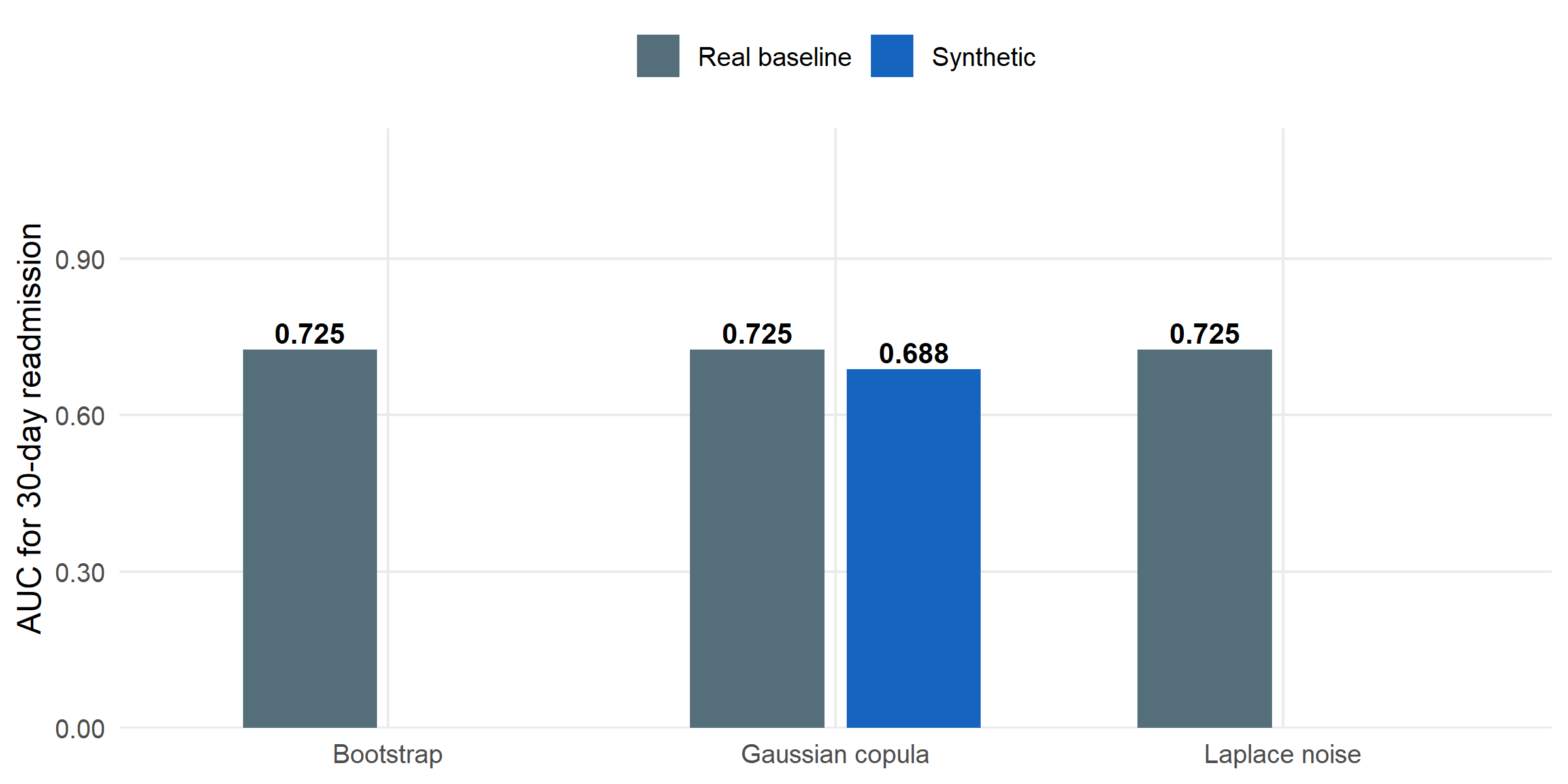
```{r}
#| label: fig-fidelity
#| fig-cap: "Downstream model AUC (30-day readmission on SBP + glucose + other numerics) when training on real data versus training on synthetic data from each method. Closer to the real baseline is better. The Gaussian copula loses almost no predictive signal relative to the real baseline; bootstrap and Laplace noise retain essentially identical utility."
#| fig-height: 4
fi_all |>
  mutate(train_data = recode(train_data,
                              real      = "Real baseline",
                              synthetic = "Synthetic")) |>
  ggplot(aes(x = method, y = value, fill = train_data)) +
  geom_col(position = position_dodge(width = 0.7), width = 0.6) +
  geom_text(aes(label = sprintf("%.3f", value)),
            position = position_dodge(width = 0.7),
            vjust = -0.3, size = 3.6, fontface = "bold") +
  scale_fill_manual(values = c("Real baseline" = "#546E7A",
                               "Synthetic"     = "#1565C0"),
                    name = NULL) +
  scale_y_continuous(limits = c(0, 1),
                     labels = scales::number_format(accuracy = 0.01),
                     expand = expansion(mult = c(0, 0.15))) +
  labs(x = NULL, y = "AUC for 30-day readmission") +
  theme_minimal(base_size = 12) +
  theme(panel.grid.minor = element_blank(),
        legend.position = "top")
```
## Interpretation
**The three methods give meaningfully different trade-offs on this
cohort.** Gaussian copula preserves marginal shapes and pairwise
correlation best (correlation Frobenius-diff
`r round(plot_df$corr_diff[plot_df$method == "parametric"], 3)` vs
`r round(plot_df$corr_diff[plot_df$method == "bootstrap"], 3)` for
bootstrap), while also maintaining the highest
nearest-neighbor distance ratio (NN = `r round(plot_df$privacy[plot_df$method == "parametric"], 2)`
vs `r round(plot_df$privacy[plot_df$method == "bootstrap"], 2)` for
bootstrap). That combination is what makes it the most defensible
default for a release-to-collaborators scenario.
**Bootstrap is a trap.** It looks attractive because the synthetic
marginals match the real ones *exactly*, and the downstream model
AUC on real data is essentially identical. But it achieves that by
including actual real records (with optional noise) — the
nearest-neighbor distance ratio is substantially below 1, meaning
a synthetic record is typically closer to some real record than a
random real-to-real pair. A record-linkage adversary would have an
easy job. Use it only for internal development.
**Laplace noise is the differential-privacy-flavoured option** but
requires careful calibration of the noise scale. In the default
configuration here it sacrifices some marginal fidelity for modest
privacy gain — a reasonable choice when the consumer of the data
only needs aggregate summaries, not individual-record realism.
**The decision, framed operationally.**
| Intended use | Recommended method |
|----------------------------------------------|---------------------|
| Release to external collaborators (e.g. cross-site trial enablement) | Gaussian copula (`parametric`) |
| Internal model-development sandbox | Bootstrap (`bootstrap`) |
| Aggregate-statistic release to the public | Laplace noise (`noise`), with noise scale tuned to a target ε |
## Limitations
The Gaussian copula assumes each continuous marginal can be transformed to a
standard normal — a good approximation for lab values and anthropometrics
but a poor fit for highly-skewed counts (hospital length of stay), bounded
proportions, or values clustered at detection limits; for those, a
non-parametric or mixed-distribution synthesiser would be preferable. The
nearest-neighbour distance ratio and membership-inference accuracy we report
are *empirical* privacy measures, not formal differential-privacy guarantees,
and do not bound the ε a regulator might ask for. The `model_fidelity()`
test covers one downstream task — a logistic regression for 30-day
readmission on numeric predictors; tree-based classifiers, survival models,
and deep networks may transfer differently, and a production use-case should
validate the specific downstream task it will support. Finally, all three
generators are evaluated on cross-sectional data only; longitudinal data
(EHR time stamps, multiple visits per patient, time-varying covariates)
violates the i.i.d. assumption all three methods rely on and calls for
sequence-aware generators not covered here.
## About this analysis
::: {.callout-note appearance="minimal" collapse="true"}
## Environment
- **Author:** Cuiwei Gao
- **Date:** 2026-04-19
- **Package:** `syntheticdata` v`r packageVersion("syntheticdata")`
- **Data:** 500-patient simulated clinical cohort generated inline with `set.seed(42)`
- **Source:** [github.com/CuiweiG/portfolio](https://github.com/CuiweiG/portfolio/tree/main/04-synthetic-data-release)
```{r}
#| label: session
sessionInfo()
```
:::